 Many processes require a dynamic point-to-point reversal movement or a point-accurate smoothing.
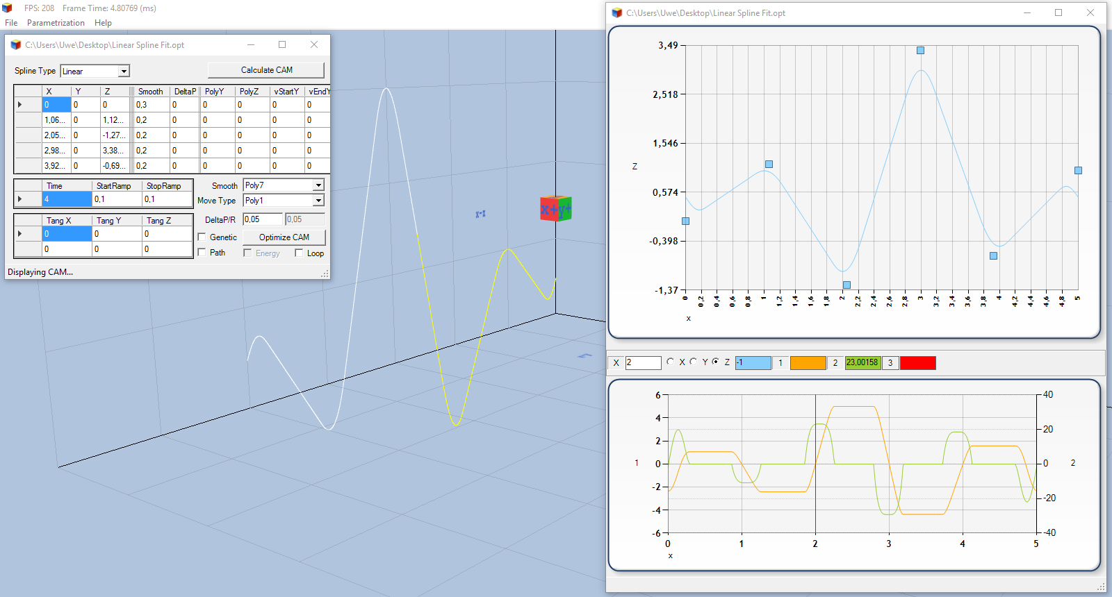
With our approach of Linear Splines for motion and our numerical solver methods, a highly dynamic, precise movement can be achieved.
 Mit dem Laden des Videos akzeptieren Sie die Datenschutzerklärung von YouTube. PGRpdiBjbGFzcz0iX2JybGJzLWZsdWlkLXdpZHRoLXZpZGVvLXdyYXBwZXIiPjxpZnJhbWUgd2lkdGg9IjU2MCIgaGVpZ2h0PSIzMTUiIHNyYz0iaHR0cHM6Ly93d3cueW91dHViZS1ub2Nvb2tpZS5jb20vZW1iZWQvdldkaVVkdkhvQXM/cmVsPTAmYW1wO3ZxPWhkMTA4MCIgZnJhbWVib3JkZXI9IjAiIGFsbG93PSJhdXRvcGxheTsgZW5jcnlwdGVkLW1lZGlhIiBhbGxvd2Z1bGxzY3JlZW49IiI+PC9pZnJhbWU+PC9kaXY+ |
The video above illustrates how a Linear Spline is simply defined via the four center reversal points (1, 1) (2, -1) (3, 3) and (4, -0.5) and this is then automatically modified so that over these reversal points is driven very dynamically. It is not necessary to stop at the reversal points, but the velocity (orange) has a zero crossing. In addition, one can also see that the acceleration (green), modeled with a polynomial of the degree 7, is capped at the respective maximum.
A similar behavior can also be achieved using Quintic Splines, if we do without a smooth third derivative and instead demand horizontal tangents at the reversal points, as shown in the video below.
|
Mit dem Laden des Videos akzeptieren Sie die Datenschutzerklärung von YouTube. PGRpdiBjbGFzcz0iX2JybGJzLWZsdWlkLXdpZHRoLXZpZGVvLXdyYXBwZXIiPjxpZnJhbWUgd2lkdGg9IjU2MCIgaGVpZ2h0PSIzMTUiIHNyYz0iaHR0cHM6Ly93d3cueW91dHViZS1ub2Nvb2tpZS5jb20vZW1iZWQveVVMeFhQMC1UUWs/cmVsPTAmYW1wO3ZxPWhkMTA4MCIgZnJhbWVib3JkZXI9IjAiIGFsbG93PSJhdXRvcGxheTsgZW5jcnlwdGVkLW1lZGlhIiBhbGxvd2Z1bGxzY3JlZW49IiI+PC9pZnJhbWU+PC9kaXY+ |
For further handling, each the resulting Linear Spline with smoothing polynomials or the pure Quintic Spline can be easily mapped to every common motion control system as a cam, so that no special manufacturer-dependent operating system is necessary.
Other processes require switching between two constant process-synchronous speeds at a precise point. Since this leads to an often significant jump in speed, you previously tried to trap such jumps on appropriate drive parameter settings. But then the reversing point isn’t reached exactly anymore
|
Mit dem Laden des Videos akzeptieren Sie die Datenschutzerklärung von YouTube. PGRpdiBjbGFzcz0iX2JybGJzLWZsdWlkLXdpZHRoLXZpZGVvLXdyYXBwZXIiPjxpZnJhbWUgbG9hZGluZz0ibGF6eSIgd2lkdGg9IjU2MCIgaGVpZ2h0PSIzMTUiIHNyYz0iaHR0cHM6Ly93d3cueW91dHViZS1ub2Nvb2tpZS5jb20vZW1iZWQvbGx1REQtQlpmVDA/cmVsPTAmYW1wO3ZxPWhkMTA4MCIgZnJhbWVib3JkZXI9IjAiIGFsbG93PSJhdXRvcGxheTsgZW5jcnlwdGVkLW1lZGlhIiBhbGxvd2Z1bGxzY3JlZW49IiI+PC9pZnJhbWU+PC9kaXY+ |
In the video above can see very well how “hard” for example the turn is on the lower reversing point without appropriate drive parameter settings and the second upper reversing point is not reached exactly with pure drive parameter adjustments. But here we want to present a solution with which such a turning maneuver is simple to implement position setpoint based with polynomials (as you can see at the first upper reversing point where the mouse points to). The user has to define only the area in which to place the maneuver and specify the exact time at which the reversing point has to be reached.
 |
A corresponding algorithm calculates a reversing polynomial (optional 5th or 7th degree), which can be integrated as a cam segment or as a table into the movement. In the picture above you can see how such a reversing polynomial can be programmed for example using JetSym STX. The calculation itself takes a maximum of one to two milliseconds even at a smaller controller from Bucher Automation AG.